Neural waves study provides evidence that brain's rhythmic patterns play key role in information processing
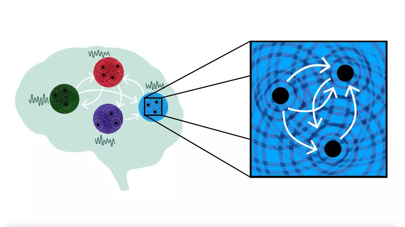
The authors of the study suggest that the brain uses the superposition & interference patterns of waves to represent and process information in a highly distributed way, exploiting the unique properties of coupled oscillator networks such as resonance and synchronization.
Papers & Code:
Code: Harmonic oscillator recurrent network (HORN) Pytorch Implementation
Overview:
High-level concepts:
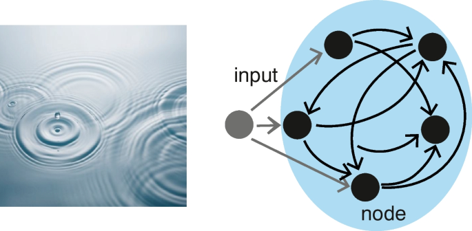
Recast neural processing as continuous‐time dynamics rather than pure feed-forward stateless layers.
Embedding physical, continuous dynamics—oscillations, waves, vortices, and damping—directly into the network’s layers unlocks powerful, implicit mechanisms for attention, multi-scale integration, and long-range memory, without the combinatorial bloat of explicit attention heads or deeper stacks.
1. Controlled Oscillations as an Inductive Bias
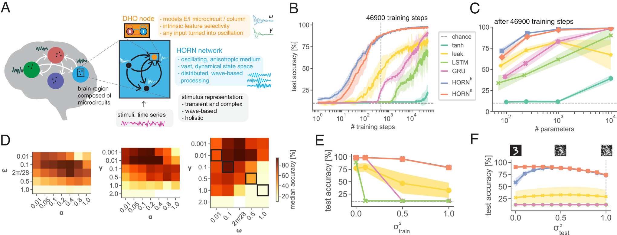
Damped Harmonic Oscillator (DHO) nodes
In model.py, each hidden unit integrates its “position” x and “velocity” y via:
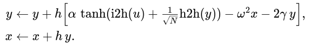
Key Insight: forcing every node into an oscillatory regime makes phase, frequency and amplitude available for coding from the very first forward pass—no need to “discover” oscillations through recurrent loops alone.
Why it matters:
- Leaky‐integrator RNNs can oscillate only indirectly (if you tweak weights).
- By baking oscillations into the node, you guarantee resonance‐based feature extraction and a rich dynamical repertoire from the start.
2. Wave‐Based Representations & Interference
Traveling waves & standing waves
- External input → local standing oscillation in each DHO
- Recurrent coupling → traveling waves that propagate, collide, and interfere
High‐Dimensional Mapping:
- Low‐dimensional time-series (e.g. pixel sweep in sMNIST) → high-dimensional spatiotemporal interference pattern across the N oscillators.
- After training, these patterns carve out stimulus‐specific trajectories in the N-dimensional state space that are linearly separable by your final
h2olayer.
Code touch-point: The record=True flag in forward() gives you rec_x_t and rec_y_t. Visualizing these (as in dynamics.py or train.py) shows exactly how different input classes sculpt different wave‐interference signatures.
3. Resonance & Intrinsic Receptive Fields
The intrinsic gain curve of each DHO node is defined as:
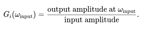
In the PNAS work, a grid‐search found optimal \omega \approx 2\pi/28 to match the dominant frequency of straight strokes in sMNIST.
Computational payoff: Nodes automatically amplify (resonate) in-band inputs—so you’re baking in priors about the signal’s spectral content at the architectural level, not just via learned weights.
How to explore in your code:
- In
dynamics.py, drive a single DHO with a pure sine wave at different frequencies. - Measure steady‐state amplitude &bar; x &bar; after transients → plot &bar; x &bar; vs. frequency.
- That’s your empirical G(\omega_{\text{in}}) curve.
4. Heterogeneity → Near‐Critical Dynamics
Biological motif: neurons/pyramidal microcircuits have tunings and delays that vary across the network.
HORN’s version: drawing each unit’s \omega_i and \gamma_i (and later, delays) from a distribution.
Why it helps:
- Expands the repertoire of possible wave‐interference patterns
- Brings network closer to a “critical” regime: balance of order/disorder, long memory tails, richer transient dynamics
Simple test in code:
- In
dynamics.pyyou already sampleomegaandgamma. Try:- Homogeneous run (all ω = ω_base, γ = γ_base) vs.
- Heterogeneous run (sampled ω, γ)
- Quantify:
- Pairwise phase‐locking values between units over time (look at how PLV distribution broadens)
- Linear separability: train a small linear SVM on the recorded
rec_x_tsnapshots and compare classification accuracy.
5. Hebbian Alignment of Backprop
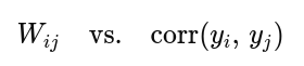
Surprising finding: gradient‐based BPTT weight updates on h2h end up correlating strongly with pre-post activity correlations—i.e. they “look Hebbian.”
Takeaway: Even though you’re minimizing a cross‐entropy loss at the readout, the recurrent weight updates reorganize the network to amplify stimulus‐specific synchrony patterns.
Next step in code:
- After an epoch of supervised training, scatter‐plot before & after training to see the emergence of a positive correlation between weight strength and firing‐correlation
6. Spontaneous → Evoked State Manifolds
Biological signature: cortex at rest floats through a “rich club” of states; stimuli transiently collapse it into a low‐variance, stimulus‐specific subspace.
HORN mimic:
- Add small random kicks to
y_t(Poisson noise) whenrecord=False - Observe via PCA on the recorded trajectories that:
- Rest: clouds of points filling a large manifold
- During input: rapid collapse to distinct clusters for each class
- After: rebound back to the resting manifold
In summary
- Oscillatory nodes give access to phase, frequency, and amplitude as first‐class coding variables.
- Wave interference provides a massively parallel, high‐dimensional embedding of inputs.
- Resonance priors let you tune the network at the architectural level to known signal statistics.
- Heterogeneity & delays enrich the dynamic repertoire and promote near‐critical, richly transient behaviors.
- Hebbian‐style learning emerges naturally even under supervised BPTT, hinting at fully unsupervised alternatives.
- Rest–stimulus manifold dynamics in HORN match key cortical phenomenology.